Graph Neural Networking Challenge 2021

Creating a Scalable Network Digital Twin

Dataset description

This website describes the datasets provided for the challenge, whose main objective is to investigate a fundamental limitation of existing Graph Neural Networks applied to data networks: Their lack of generalization capability to larger networks.

Please, find the download links at the bottom of this website. Although we first recommend reading carefully all the information below.

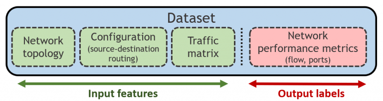
The datasets are generated with OMNet++, a discrete event packet-level network simulator. Each sample (Fig. 1) simulates a network scenario, defined by: (i) a network topology, (ii) a routing configuration, and (iii) a source-destination traffic matrix, and it is labeled with network performance metrics obtained by the simulator, including per-source-destination performance measurements (mean per-packet delay, jitter and loss), and port statistics (e.g., queue utilization, avg. packet loss). Note that this challenge focuses only on the prediction of the mean per-packet delay on each source-destination path.

At the beginning of the challenge, we provide two datasets for training and validation, that participants can use to develop their solutions. As the challenge is focused on scalability, the validation dataset contains samples of networks considerably larger (51-300 nodes) than those of the training dataset (25-50 nodes). Likewise, the test dataset will be released at the end of the challenge (tentatively, on Sep 15th), just before the evaluation phase starts, and it will contain samples following a similar distribution to those of the validation dataset.

Note that solutions can only be trained on samples of the training dataset. Data augmentation techniques are allowed as long as they only use data from the training dataset. The validation dataset should be exclusively used to evaluate the model. At the end of the challenge, we will check if winning solutions comply with this rule by reproducing the solution.

The training dataset contains samples simulated in topologies of 25, 30, 35, 40, 45, and 50 nodes, including two different network topologies for each topology size.

The validation dataset contains samples on larger network topologies. Particularly, they contain two different topologies for each of the following network sizes: 50, 55, 60, 65, 70, 75, 80, 85, 90, 95, 100, 110, 120, 130, 140, 150, 160, 170,180 ,190, 200, 220, 240, 260, 280, and 300.

All the topologies have been artificially generated using the Power-Law Out-Degree Algorithm described in [1], where the ranges of the α and β parameters of the algorithm have been extrapolated from real topologies of the Internet Topology Zoo repository [2]. Likewise, all nodes implement only one FIFO queue on each output port.

The link capacity is individually selected according to the maximum traffic intensity that the network can support in our simulations, assuming a limited packet loss rate (<3% approx.). In each path, packets are generated with a Poisson process and the packet size is modeled with a binomial distribution.

For each topology, we generate different routing configurations, which are generated as variations of the shortest path routing scheme. In the validation dataset, we also generate some routing configurations with artificially longer paths, to test the capabilities of solutions to generalize to longer paths.

Validation dataset:

One important factor when scaling to large networks is to consider that they will present to main features with respect to the smaller networks: (i) longer end-to-end paths (as the network diameter increases), and (ii) larger link capacities (as central links usually carry more aggregated traffic). The validation dataset comprises three subsets intended to evaluate separately these two features (longer paths and larger link capacities), and the combination of them. All these 3 subsets contain the same number of samples (1.080 samples each one), which are simulated on all the topology sizes mentioned above (i.e., 50-300 nodes):

Subset 1:

This subset focuses individually on the longer paths feature. It contains samples where the routing configuration has long source-destination paths artificially generated. However, link capacities are in the same range as in the training dataset. Note that in samples of this subset not all the potential source-destination paths transmit traffic, only some of them that are particularly long.

Subset 2:

This subset focuses individually on the larger link capacity feature. We use variants of shortest path routing policy, and all the src-dst pairs transmit traffic. As a result the traffic aggregated on links is considerably larger than in the smaller networks of the training dataset. To support this traffic aggregates, some links of these topologies have larger capacities than the maximum observed in the training dataset.

Subset 3:

This subset covers the two features mentioned above: longer paths and larger link capacities. To do so, we generate routing schemes with longer paths. However, unlike subset 1, in this subset all src-dst pairs transmit traffic. As a result, link capacities are larger than in the training dataset to support the traffic aggregates on these scenarios.

One good approach for participants to develop their solutions would be to first focus individually on each feature: longer paths (subset 1) and larger link capacities (subset 2), and then test the solution in samples combining both features (subset 3).

Processing the dataset

It is highly recommended to use the API provided [here] to easily read and process samples from the dataset. However, if you prefer to use directly the raw data, you can find the description of the dataset format below.

The root directory of datasets (compressed files) contains a folder for each topology size. Each of these directories can be considered as a subdataset with the ‘routings’ directory where routing configuration files are stored. These files include a line for each src-dst path, defined as a list of the nodes that form the path.

In the ‘graphs’ directory we locate the topologies and their features associated. Each topology file describes the nodes and links of the topology in Graph Modeling Language (GML). This file can be processed with the networkx library using the read_gml method:

G= networkx.read_gml(topology_file, destringizer=int)

Finally, we have a set of compressed files with 25 / 10 simulation samples each one (training / validation). Each of these files contain the following data:

input_files.txt: Each line of this file contains the simulation number, the topology file, and the routing file used for that simulation.

traffic.txt: Contains the traffic parameters used by the simulator to generate the traffic for each iteration. At the beginning of each line we have the maxAvgLambda selected for this iteration. This parameter is separated from the rest of the information with the ‘|’ character. The rest of the line corresponds to the parameters used to generate the traffic for each path. Paths information are separated with semicolon (;) and the parameters used for those paths are separated with commas (,). The parameters of each path depend on the time an packet size distribution used and is structured as follows:

< time_distibution >,< equivalent_lambda >, < time_dist_param_1 >,..,< time_dist_param_n >,< size_distibution >, < avg_pkt_size >, < size_dist_param_1 >,..,< size_dist_param_n >< ToS >.

For this dataset the time_distribution is always Poisson (i.e., =0) and the size distribution is binomial (i.e., =2).

The rest of parameters for the Poisson/Exponential distribution are:
• Avg number of packets per time unit considering packets of avg_pkt_size.
• Exponential max factor: Factor used to define an upper bound for exponential distributions. The upper bound is defined as: ‘ExpMaxFactor’* equivalent_lambda.

The rest of parameters for the binomial distribution are:
• Packet size 1: First packet size option (bits).
• Packet size 2: Second packet size option (bits).

simulationResults.txt: Contains the measurements obtained by our network simulator for every sample. Each line in ‘simulationResults.txt’ corresponds to a simulation using the topology and a routing specified in the ‘input_files.txt’, and the input traffic matrices specified in the ‘traffic.txt’ file.
At the beginning of the line, and separated by “|”, there are global network statistics separated by commas (,). These global parameters are:
1. global_packets: Number of packets transmitted in the network per time unit (packets/time unit).
2. global_losses: Packets lost in the network per time unit (packets/time unit).
3. global_delay: Average per-packet delay over all the packets transmitted in the network (time units)After the “|” and separated by semicolon (;) we have the list of all path. Finally the metrics of the related to a path are separated by commas (,). Likewise, the different measurements (e.g., delay, jitter) for each path are separated by commas (,). So, to obtain a pointer to the metrics of a specific path from ‘node_src’ to ‘node_dst’, one can split the CSV format considering the semicolon (;) as separator:list_metrics[src_node*n+dst_node] = path_metrics (from src to dst)
  Where ‘list_metrics’ is the array of strings obtained from splitting the line after the “|” character using semicolon. Note that in a topology with ‘n’ nodes, nodes are enumerated in the range [0, n-1]
  This pointer will return a list of measurements for a particular src-dst path. In this list measurements are separated by comma (,) and provide the following measurements:
  1. Bandwidth (in kbits/time unit) transmitted in each source-destination pair in the network.
  2. Number of packets transmitted in each src-dst pair per time unit.
  3. Number of packets dropped in each src-dst pair per time unit.
  4. Average per-packet delay over the packets transmitted in each src-dst pair (in time units).
  5. Average neperian logarithm of the per-packet delay over the packets transmitted in each src-dst pair (in time units). This is avg(Ln(packet_delay)).
  6. Percentile 10 of the per-packet delay over the packets transmitted in each src-dst pair (in time units).
  7. Percentile 20 of the per-packet delay over the packets transmitted in each src-dst pair (in time units).
  8. Percentile 50 (median) of the per-packet delay over the packets transmitted in each src-dst pair (in time units).
  9. Percentile 80 of the per-packet delay over the packets transmitted in each src-dst pair (in time units).
  10. Percentile 90 of the per-packet delay over the packets transmitted in each src-dst pair (in time units).
  11. Variance of the per-packet delay (jitter) over the packets transmitted in each source-destination pair.

stability.txt: Contains some extra information used to evaluate the status of the dataset. The more relevant parameter from this file is the simulation time required to reach the stability condition which, for each simulation, is the first element of the line.
linkUsage.txt: For each src-dst pair, if there is a link between them, it contains the outgoing port statistics separated by comma (,) or -1 otherwise. Each src-dst port information is separated from the rest by semicolon (;). The list of parameters for each src-dst outgoing port is:

Average utilization of the outgoing port (in the range [0,1]).
Average packet loss rate in the outgoing port (in the range [0,1]).
Average packet length of the packets transmitted through the outgoing port.
Average utilization of the first queue of the outgoing port (in the range [0,1]).
Average packet loss rate in the first queue of the outgoing port (in the range [0,1]).
Average port occupancy (service and waiting queue) of the first queue of the outgoing port.
Maximum queue occupancy of the first queue of the outgoing port.
Average packet length of the packets transmitted through the first queue of the outgoing port.

Download datasets

File	Size	MD5SUM
Training dataset	6,9 GB	43594151cbddd968a5ebc38614999cd5
Validation dataset	2,2 GB	cd1da75419add2700607bbd44d4b0a66
Test dataset	524 MB	ddf346bedff4d0dfafc1591e89e0914a
Test dataset with labels	1,2 GB	555d88b091a66c716a1b73cf2d28ccd4

[1] Generating network topologies that obey power laws. IEEE. Global Telecommunications Conference 2000. C.R. Palmer & J.G. Steffan

[2] The Internet Topology Zoo. http://www.topology-zoo.org