
Graph Neural Networking Challenge 2023
Creating a Network Digital Twin with Real Network Data
Creating a Network Digital Twin with Real Network Data
Test dataset: download
Datasets
The present edition of the challenge includes two datasets that collectively exceed 400GB in size. This is because, in addition to performance metrics, users are provided with information about each transmitted packet. To facilitate the download process, the datasets have been divided into several compressed files, each approximately 5GB in size.
The first file, which is not numbered, contains the topology, routing, and performance files. The remaining files, whos file name ends with pkts_traces plus a number, contain the packet level information for each of the samples. This division allows users to start working without having to download all the files at once.
To ensure proper functionality, it is essential to extract the compressed files into the same directory.
Please find below the links to download the datasets.
You can start participating in the challenge by just downloading two files:
– gnnet-ch23-dataset-mb.zip
– gnnet-ch23-dataset-cbr-mb.zip
gnnet-ch23-dataset-mb:
gnnet-ch23-dataset-cbr-mb:
gnnet-ch23-test-dataset:
Testbed
The following figure provides an overview of the testbed and in what follows we describe each of the components:
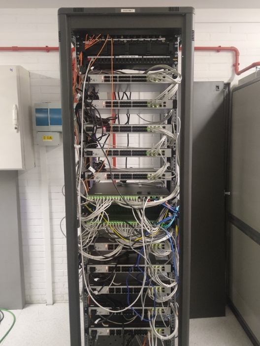
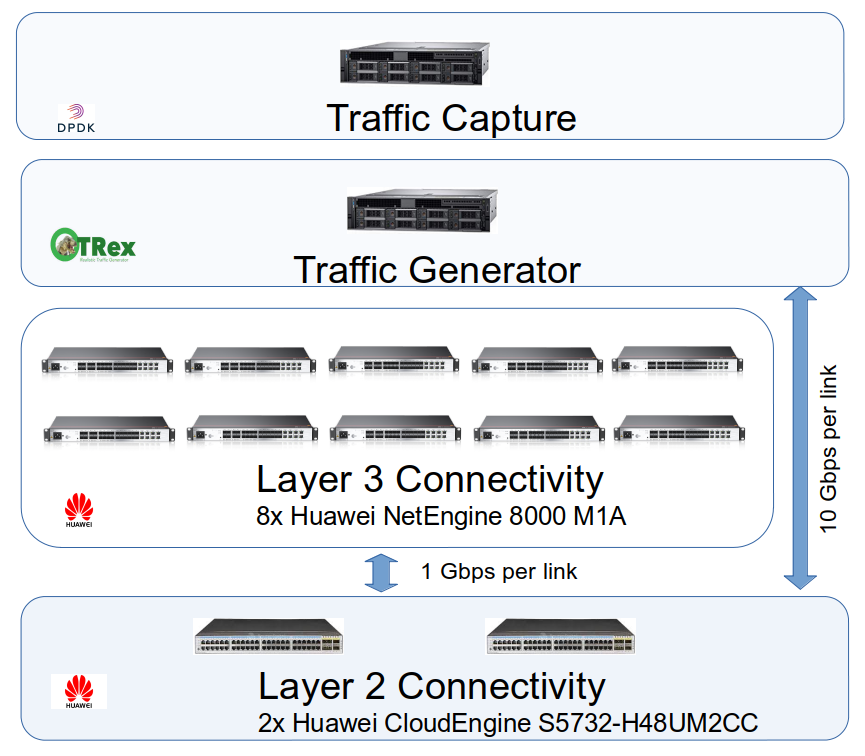
Network Equipment:
Our network testbed comprises 8 hardware router (Huawei NetEngine 8000 M1A), each utilizing 6 ports connected via 2 hardware switches with 48 ports at 1 Gbps. A traffic generator (T-REX) is attached to the testbed through 10Gbps ports with the switches. Additionally, two ports of 40 Gigabit Ethernet are used to interconnect both switches in Ethernet Trunk mode. This configuration allows us to build any physical topology with up to 8 nodes, with a node degree ranging from 1 to 5 (one of the ports is reserved for traffic generation), and configure routing policies as needed.
Network topology:
The dataset comprises 11 randomly generated topologies ranging from 5 to 8 nodes. Adjacent routers are interconnected through switches using dedicated ports. The switch port is configured as an access port, this is a unique VLAN used for traffic exchanged between the adjacent routers. The traffic generator is connected to the switch using a trunk port. This trunk port ensures that traffic intended for each router is separated from the others using VLANs (Virtual Local Area Networks). Traffic between switches is sent through a 2x40Gb link. This port is configured as a trunk port and has VLAN isolation.
Routing:
For each of the selected topologies we use 10 different routings. Each routing is based on a destination-based policies that are variations of the shortest path.
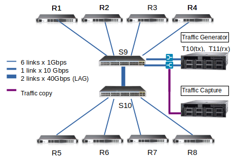
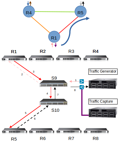
The figure above (left) shows how the different network devices are interconnected. The figure above (right) shows an example of the physical path followed by a single flow originating at router 1 with destination router 2. Note that the delay of the flow is from the egress to the ingress of the Traffic Generation device, and that hops through the switches several times.
Traffic Generation:
We use the open-source project T-Rex to generate traffic. Specifically, we generate 1 or 2 flows per path, which can be Constant Bit Rate (CBR) or Multi Burst (MB).
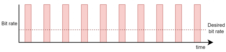
Constant-Bit Rate (CBR): Traffic is sent in short and intense bursts (at line rate), followed by periods of no transmission. See the figure below for an illustrated example.
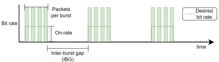
Multi-burst (MB): Traffic is sent in bursts defined by three parameters: packets per burst, on-rate and inter-burst gap. The figure below shows an illustrated example.
Each experiment has a duration of 10 seconds, with the first 5 seconds being discarded to avoid the transient-state. Note that all packets of a flow have the same size. Also note that lost packets will show-up in the output packet trace but with no delay associated.
T-Rex generates packets at line-rate (10Gbps) and then stops to meet the requested bandwidth, this process occurs each millisecond. This approach results in a bursty traffic pattern that becomes smoother at higher loads and when multiplexing several flows.
The server we use for traffic generation is equipped with an Intel X710-DA4 that has four 10Gbps NICs. We associate every two ports with one instance of T-Rex and connect them to one of the switches.
Traffic Measurement:
In order to measure the delay we use an optical splitter at the fibers that interconnects the traffic generator with the testbed. With this, we create an exact copy of the traffic both at ingress and egress. This traffic is processed by a set of Mellanox ConnectX-5 cards. These cards support hardware timestamping, which is a necessary feature to measure delays accurately. We use DPDK to process the traffic and compute the delay.
Two different datasets will be provided for this challenge: (i) training/validation and (ii) test. Each dataset includes the average per-flow delay of thousands of samples. Each sample is an instance of a topology, routing, and a set of flows with different rates. The test dataset is equivalent but it will not include the output label (per-flow delay).
Additional considerations
In what follows we provide a set of additional considerations, this is included for transparency but most likely it is irrelevant for participants:
- Packet loss: Lost packets will show-up in the output packet trace but with no delay associated.
- All packets in the same flow follow the same routing path. In the scenarios where there are multiple flows sharing the same source and destination, they will also share the same routing path.
- Two traffic generators are used to generate traffic. Each traffic generator is an independent machine, whose clocks are not synchronized (i.e. the timestamps values generated by one traffic generator cannot be compared with the timestamp values generated by the other). But since all packets from the same flow are generated by the same traffic generator, we can compare the timestamps of packets within the same flow.
- There can be multiple physical connections between the switches and routers.
- Link identifiers are defined by a 3-way tuple between the source, destination, and the port number used by the source.
- Each physical link has two identifiers, one provided by each end of the link. For example, given a link between router 1 and switch 2, the router will identify the link as “(r1,s2,0)” (port number 0), while the switch will identify it as “(s2,r1,3)” (port number 3).
- All links are full duplex.
- Due to the nature of the topology of the testbed, the links originating from the Traffic Generator and ending on the switch, will never be congested. As a result, their impact on the packet delay is minimal and can be safely discarded. Note that is DOES NOT apply in the other direction, links originating from the switch and end on
the Traffic Generator.
ANNEX:
RAW details of the datasetThis ANNEX details the RAW format of the dataset
The root directory of the decompressed dataset contains the ‘graphs’ directory where we locate the topologies and their features associated. Each topology file describes the nodes and links of the topology in Graph Modeling Language (GML). This file can be processed with the networkx library using the read_gml method:
G= networkx.read_gml(topology_file, destringizer=int)
There are two type of topology files:
- graph_<topo_name>.txt: Describe the layer 3 topology. The topology only contains routers.
- l2_graph-<topo_name>.txt: Describe the physical links interconnecting traffic generators, routers and switches.
The ‘routings’ directory where routing configuration files are stored. Each file corresponds to a specific routing. Within each file, each line represents a path, expressed as a sequence of nodes.
In this folder, you can also find the layer2 path descriptor for each topology (l2_routing<topology_name>.txt). The lines of this file describe the port sequence between adjacent layer 3 devices (traffic generators and routers). Ports are identified as a string with the following format:
<src node type><src node id>-<next hop node type><next hop node id>-<port count>
<src node type><src node id> can be used to identify the elements in the network. The node type can be:
- ‘t’: Traffic generator
- ‘r’: Router
- ‘s’: Switch
Finally, in the routing path, we have the tg_per_path-<topology>.txt files which indicates the source and destination traffic generator used per each path. Note that a path is described as the src-dst router id: <src router id> <dst router id> <tx traffic generator> <rx traffic generator>
The last folder is pkts_info. In this folder we can find, a pickle file per sample. The object of the pickle file is a numpy matrix. For each src-dst returns a dictionary where the key is a ToS and the value is a list of lists. There is one list per flow using the same order than the flows described in traffic matrix or the performance matrix (described later). The list contain information for each packet of the flow. This information is stored as a tuple of three elements: the generation timestamp in nanoseconds (not to be confused with other elements of the sample being described in seconds), the packet size in bits, and the delay in seconds. If a packet has been dropped, the delay value is not present in the tuple.
Thus, assuming pinfo is the pkts_info object of a sample, pinfo[src,dst][tos][numflow] returns the list of tuples with per packet information of packets transmitted in the flow numflow of the src-dst path with ToS tos.
To load a pickle file:
import pickle
pkt_info_object = pickle.load(open(<pickle file>, ‘rb’))
Finally, we have a set of compressed files with 25 experiment samples each one. Each of these files contain the following data:
input_files.txt: Each line of this file contains the experiment number, the topology file, the routing file, the layer 2 topology file, the layer 2 paths file and the src-dst path to traffic generators file.
tm/tm-<sample_id>.txt: Contains the parameters used by the traffic generator to generate the traffic for the sample_id run. The first line of the file is the max_link_load which is used to define the maximum link load when generating the traffic matrix of the scenario and It is an indicator of the load of the network. The following lines are the traffic descriptors per each path. Using semicolon to split the content of these lines, we have the src and dst node of the path and then a set of flows descriptors. The parameters describing the flow are separated by comas.
- Constant Bit Rate (CBR) flow:
- Packet size in bytes
- Bandwidth rate in bps
- ToS. Always 0 for these datasets.
- Multi Burst (MB) flow:
- Packet size in bytes
- Bandwidth rate in bps during the burst
- Number of packets of each burst
- Number of burst during the experiment (this value can be ignored)
- Inter burst gap in microseconds
- Inter stream gap in microseconds. Time to start the first burst. Always 0 for these datasets.
- ToS. Always 0 for these datasets.
experimentResults.txt: Contains the measurements per path obtained by our network testbed for every sample. Each line in ‘experimentResults.txt’ corresponds to an experiment using the topology and a routing specified in the ‘input_files.txt’, and the input traffic parameters specified in the ‘tm/tm-<sample_id>.txt’ file. At the beginning of the line, and separated by “|”, there are global network statistics separated by commas (,). These global parameters are:
- capture_time: The experiment takes 10 seconds to complete but only the last captur_time seconds are captured and processed.
- global_packets: Number of packets transmitted in the network per time unit (packets/time unit).
- global_losses: Packets lost in the network per time unit (packets/time unit).
- global_delay: Average per-packet delay over all the packets transmitted in the network (seconds).
After the “|” and separated by semicolon (;) we have the list of all path. Finally the metrics of the related to a path are separated by commas (,). Likewise, the different measurements (e.g., delay, jitter) for each path are separated by commas (,). So, to obtain a pointer to the metrics of a specific path from ‘node_src’ to ‘node_dst’, one can split the CSV format considering the semicolon (;) as separator:
list_metrics[src_node*n+dst_node] = path_metrics (from src to dst)
Where ‘list_metrics’ is the array of strings obtained from splitting the line after the “|” character using semicolon. Note that in a topology with ‘n’ nodes, nodes are enumerated in the range [0, n-1] This pointer will return a list of measurements for a particular src-dst path. In this list measurements are separated by comma (,) and provide the following measurements:
- Average traffic rate (in bits/s) transmitted in each source-destination pair in the network.
- Number of packets transmitted in each src-dst pair per second.
- Number of packets dropped in each src-dst pair per second.
- Average per-packet delay over the packets transmitted in each src-dst pair (in seconds).
- Average natural logarithm of the per-packet delay over the packets transmitted in each src-dst pair. This is avg(Ln(packet_delay)).
- 10th percentile of the per-packet delay over the packets transmitted in each src-dst pair (in seconds).
- 20th percentile of the per-packet delay over the packets transmitted in each src-dst pair (in seconds).
- 50th percentile (median) of the per-packet delay over the packets transmitted in each src-dst pair (in seconds).
- 80th percentile of the per-packet delay over the packets transmitted in each src-dst pair (in seconds).
- 90th percentile of the per-packet delay over the packets transmitted in each src-dst pair (in seconds).
- Variance of the per-packet delay (jitter) over the packets transmitted in each src-dst pair.
- Average packet size over the packets transmitted on the path (in bits)
- 10th percentile of the per-packet size over the packets transmitted in each src-dst pair (in bits).
- 20th percentile of the per-packet size over the packets transmitted in each src-dst pair (in bits).
- 50th percentile of the per-packet size over the packets transmitted in each src-dst pair (in bits).
- 80th percentile of the per-packet size over the packets transmitted in each src-dst pair (in bits).
- 90th percentile of the per-packet size over the packets transmitted in each src-dst pair (in bits).
- Variance of the per-packet size over the packets transmitted in each src-dst pair.
If the sample have more than one flow per path, then the experimentResultsFlow.txt is also included.
experimentResultsFlow.txt: Contains the measurements per flow obtained by our network testbed for every sample. Each line in ‘experimentResultsFlow.txt’ corresponds to an experiment using the topology and a routing specified in the ‘input_files.txt’, and the input traffic parameters specified in the ‘tm/tm-<sample_id>.txt’ file.
We use semicolon (;) to separate paths in the line and colon(:) to separate flows in a path. Finally the metrics of the related flow are separated by commas (,). Likewise, the different measurements (e.g., delay, jitter) for each flow are separated by commas (,). So, to obtain a pointer to the metrics of a specific flow from ‘node_src’ to ‘node_dst’, one can split the CSV format considering the semicolon (;) as separator:
list_metrics[src_node*n+dst_node] = path_metrics (from src to dst)
Where ‘list_metrics’ is the array of strings obtained from splitting the line using semicolon. The obtained string is then spitted again using colon(:) to obtain the list of flows.
Note that in a topology with ‘n’ nodes, nodes are enumerated in the range [0, n-1] This pointer will return a list of measurements for a particular flow of src-dst path. In this list measurements are separated by comma (,) and provide the same metrics described per path in the experimentResults.txt file.